출처: 네이버 부스트코스 인공지능(AI) 기초 다지기 3. 기초 수학 첫걸음
<목차>
1. Creation function
- arange
- zeros, ones, empty, something_like
- identity, eye, diag
- random sampling
2. Operation function
- sum (mathematical funcs)
- axis
- mean, std
- concatenate
3. array operations
- operations b/t arrays, element-wise operations
- dot product
- transpose
- broadcasting
- Creation function
Arange
- array의 범위를 지정하여 값의 list를 생성하는 명령어
np.arange(10) #array([0, 1, 2, 3, 4, 5, 6, 7, 8, 9])
np.arange(0, 5, 0.5) #array([ 0. ,  0.5,  1. ,  1.5,  2. ,  2.5,  3. ,  3.5,  4. ,  4.5])
zeros / np.zeros(shape, dtype, order)
0으로 가득찬 ndarray 생성
np.zeros(shape=(10,), dtype=np.int8) # 10 - zero vector 생성
#array([0, 0, 0, 0, 0, 0, 0, 0, 0, 0], dtype=int8)
ones / np.ones(shape, dtype, order)
1로 가득찬 ndarray 생성
np.ones(shape=(10,), dtype=np.int8)
array([1, 1, 1, 1, 1, 1, 1, 1, 1, 1], dtype=int8)
empty
shape만 주어지고 비어있는 ndarray 생성 (memory initialization이 되지 않음)
np.empty(shape=(10,),dtype = np.int8)
#array([ -16,   62, -116,  -96,   64,    1,    0,    0,    0,    0], dtype=int8)

np.empty((3,5))
'''
array([[0., 0., 0., 0., 0.],
       [0., 0., 0., 0., 0.],
       [0., 0., 0., 0., 0.]])
'''
something(zeros, ones,empty)_like
기존 ndarray의 shape만큼의 1,0 또는 empty array를 반환
test_matrix = np.arange(30).reshape(5,6)
np.zeros_like(test_matrix)
'''
array([[0, 0, 0, 0, 0, 0],
       [0, 0, 0, 0, 0, 0],
       [0, 0, 0, 0, 0, 0],
       [0, 0, 0, 0, 0, 0],
       [0, 0, 0, 0, 0, 0]])
'''

test_matrix2 = np.arange(30).reshape(5,6)
np.ones_like(test_matrix2)
'''
array([[1, 1, 1, 1, 1, 1],
       [1, 1, 1, 1, 1, 1],
       [1, 1, 1, 1, 1, 1],
       [1, 1, 1, 1, 1, 1],
       [1, 1, 1, 1, 1, 1]])
'''
identity
단위 행렬(i 행렬)을 생성함
np.identity(n=3, dtype=np.int8)
'''
array([[1, 0, 0],
       [0, 1, 0],
       [0, 0, 1]], dtype=int8)
'''

np.identity(5)
'''
array([[ 1.,  0.,  0.,  0.,  0.],
       [ 0.,  1.,  0.,  0.,  0.],
       [ 0.,  0.,  1.,  0.,  0.],
       [ 0.,  0.,  0.,  1.,  0.],
       [ 0.,  0.,  0.,  0.,  1.]])
'''
eye
대각선이 1인 행렬 생성, k 값을 사용해 시작 index 변경 가능
np.eye(3)
'''
array([[ 1.,  0.,  0.],
       [ 0.,  1.,  0.],
       [ 0.,  0.,  1.]])
'''

np.eye(3,5,k=2)
'''
array([[ 0.,  0.,  1.,  0.,  0.],
       [ 0.,  0.,  0.,  1.,  0.],
       [ 0.,  0.,  0.,  0.,  1.]])
'''
diag
대각 행렬의 값을 추출함

random sampling
데이터 분포에 따른 sampling으로 array 생성
- uniform : 균등분포
- normal : 정규분포
np.random.uniform(0,1,10).reshape(2,5)
'''
array([[ 0.67406593,  0.71072857,  0.06963986,  0.09194939,  0.47293574],
       [ 0.13840676,  0.97410297,  0.60703044,  0.04002073,  0.08057727]])
'''

np.random.normal(0,1,10).reshape(2,5)
'''
array([[ 1.02694847,  0.39354215,  0.63411928, -1.03639086, -1.76669162],
       [ 0.50628853, -1.42496802,  1.23288754,  1.26424168,  0.53718751]])
'''- Operation functions
sum
ndarray의 element들 간의 합을 구함
test_array = np.arange(1,11) #array([ 1,  2,  3,  4,  5,  6,  7,  8,  9, 10])
test_array.sum(dtype=np.float) #55.0
axis
모든 operation func를 실행할 때 기준이 되는 dimension 축
새롭게 생기는 shape이 axis = 0이 됨
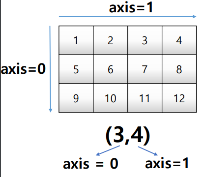
test_array = np.arange(1,13).reshape(3,4)
'''
array([[ 1,  2,  3,  4],
       [ 5,  6,  7,  8],
       [ 9, 10, 11, 12]])
'''
test_array.sum() #78
test_array.sum(axis=1) #row별로 합해라
#array([10, 26, 42])
test_array.sum(axis=0) #col 별로 합해라
#array([15, 18, 21, 24])

third_order_tensor.sum(axis=2)
'''
array([[10, 26, 42],
       [10, 26, 42],
       [10, 26, 42]])
'''

third_order_tensor.sum(axis=1)
'''
array([[15, 18, 21, 24],
       [15, 18, 21, 24],
       [15, 18, 21, 24]])
'''

third_order_tensor.sum(axis=0)
'''
array([[ 3,  6,  9, 12],
       [15, 18, 21, 24],
       [27, 30, 33, 36]])
'''
mean
ndarray의 element 간의 평균을 반환
std
ndarray의 element 간의 표준편차을 반환
test_array = np.arange(1,13).reshape(3,4)
'''
array([[ 1,  2,  3,  4],
       [ 5,  6,  7,  8],
       [ 9, 10, 11, 12]])
'''
test_array.mean(), test_array.mean(axis=0)
#(6.5, array([ 5.,  6.,  7.,  8.]))
test_array.std(), test_array.std(axis=0)
'''
(3.4520525295346629,
array([ 3.26598632,  3.26598632,  3.26598632,  3.26598632]))
'''
그 외에도
- exp, expm1, exp2, log, log10, log1p, log2, power, sqrt
- sin, cos, tan, acsin, arccos, atctan
- sinh, cosh, tanh, acsinh, arccosh, atctanh
concatenate
numpy array를 합치는 함수

a = np.array([1, 2, 3])
b = np.array([2, 3, 4])
np.vstack((a,b))
'''
array([[1, 2, 3],
       [2, 3, 4]])
'''

a = np.array([ [1], [2], [3]])
b = np.array([ [2], [3], [4]])
np.hstack((a,b))
'''
array([[1, 2],
       [2, 3],
       [3, 4]])
'''

a = np.array([[1, 2, 3]])
b = np.array([[2, 3, 4]])
np.concatenate( (a,b) ,axis=0)
'''
array([[1, 2, 3],
       [2, 3, 4]])
'''
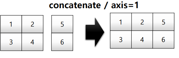
a = np.array([[1, 2], [3, 4]])
b = np.array([[5, 6]])

np.concatenate( (a,b.T) ,axis=1)
'''
array([[1, 2, 5],
       [3, 4, 6]])
'''- array operations
Operations b/t arrays
numpy는 array 간의 사칙 연산 지원
Element-wise operations
array간 shape이 같을 때 일어나는 연산
test_a = np.array([[1,2,3],[4,5,6]], float)
test_a + test_a # Matrix + Matrix 연산
'''
array([[  2.,   4.,   6.],
       [  8.,  10.,  12.]])
'''

test_a * test_a # Matrix내 element들 간 같은 위치에 있는 값들끼리 연산
'''
array([[  1.,   4.,   9.],
       [ 16.,  25.,  36.]])
'''
Dot product
numpy array 곱할 때
test_a = np.arange(1,7).reshape(2,3)
test_b = np.arange(7,13).reshape(3,2)
test_a.dot(test_b)
'''
array([[ 58,  64],
       [139, 154]])
'''
Transpose
행과 열을 바꿀 때 (T attribute 사용 가능)
test_a = np.arange(1,7).reshape(2,3)
'''
array([[1, 2, 3],
       [4, 5, 6]])
'''

test_a.transpose()  # test_a.T 와 동일
'''
array([[1, 4],
       [2, 5],
       [3, 6]])
'''

test_a.T.dot(test_a) # Matrix 간 곱셈
'''
array([[17, 22, 27],
       [22, 29, 36],
       [27, 36, 45]])
'''
broadcasting
shape이 다른 배열 간 연산을 지원하는 기능
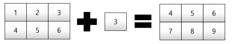
test_matrix = np.array([[1,2,3],[4,5,6]], float)
scalar = 3
test_matrix + scalar # Matrix - Scalar 덧셈
'''
array([[ 4.,  5.,  6.],
       [ 7.,  8.,  9.]])
'''

'전공공부 > 인공지능' 카테고리의 다른 글
| 부스트코스 인공지능(AI) 다지기 -6 : 벡터 (0) | 2022.07.19 |
|---|---|
| Numpy 3편 (0) | 2022.07.19 |
| Numpy (0) | 2022.07.18 |
| [코세라] Fundamentals of CNNs and RNNs (RNN) (0) | 2021.08.05 |
| [코세라] Fundamentals of CNNs and RNNs (CNN) (0) | 2021.08.05 |