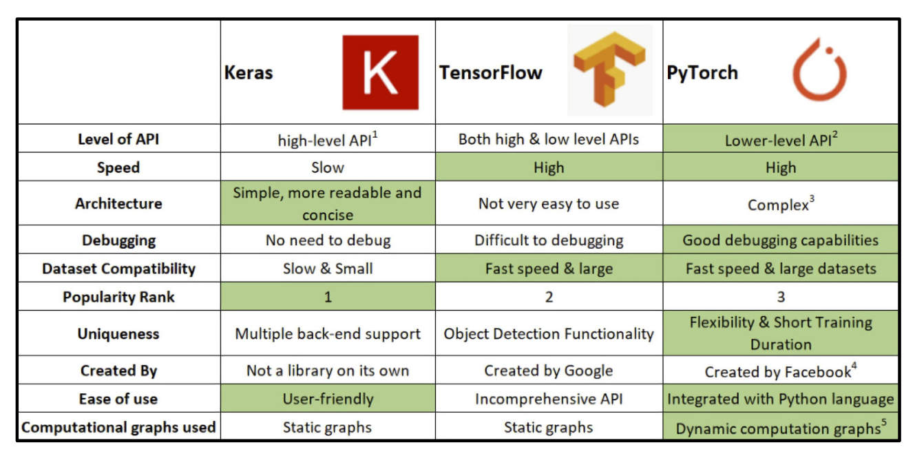
1. 딥러닝 프레임워크의 종류
2. PyTorch의 기본적인 작동 구조
- view와 reshape의 차이
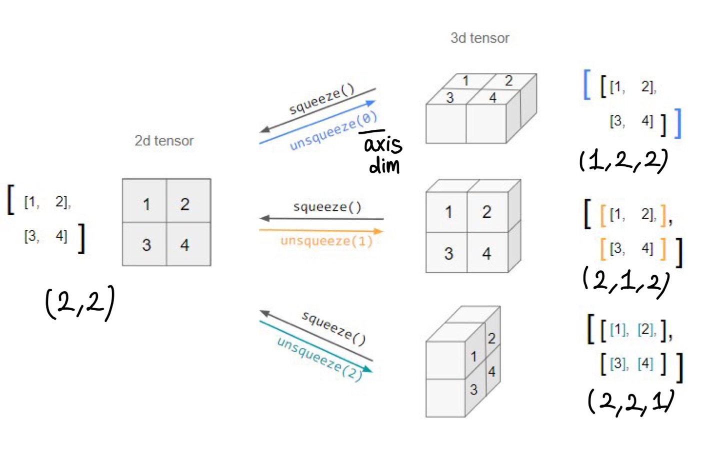
- unsqueeze, squeeze
- dot와 mm의 차이
- mm과 matmul의 차이: broadcasting
** Autograd
미분을 하려면 backward propagation을 해야함. 그러기 위해서는 먼저 현재 데이터를 그래프로 표현해야함.
이때 어떤식으로 표현하느냐?
| TF | Google static graphs Define and run : 그래프를 먼저 정의 -> 실행 시점에 데이터 feed(데이터를 넣어줌) production, cloud, multi-GPU에서 장점 production과 scalability의 장점 |
| PyTorch Numpy + AutoGrad - Numpy 구조를 가지는 Tensor 객체로 array 표현 - 자동 미분을 지원하여 Deep Learning 연산을 지원 - 다양한 형태의 DL 지원 (ex. dataset, multi-GPU) |
Facebook dynamic computaion graphs(DCG) Define by run : 실행을 하면서 그래프를 생성하는 방식 - 즉시 확인 가능 -> pythonic code - GPU support 개발 과정 디버깅이 쉬움- 구현에서의 장점 |
- 기본적으로 tensor가 가질 수 있는 data type은 numpy와 동일하고 사용법이 그대로 적용됨
- 기본적인 tensor의 operations는 numpy와 동일
.flatten(), .ones_like(), .numpy(), .shape, .dtype
view: reshape과 동일하게 tensor의 shape를 변환
sequeeze: 차원의 개수가 1인 차원을 삭제(압축)
unsqueeze: 차원의 개수가 1인 차원을 추가
view와 reshape은 contiguity 보장의 차이
view는 복사를 한 게 아니라 메모리 주소를 그대로 사용하고 형태만 바꾼 것임 view를 써라
a= torch.zeros(3, 2)
b=a.view(2,3)
a.fill_(1)
print(a)
print(b)
'''
tensor([[1., 1.],
        [1., 1.],
        [1., 1.]])
tensor([[1., 1., 1.],
        [1., 1., 1.]])
'''

a=torch.zeros(3,2)
b=a.t().reshape(6)
a.fill_(1)
print(a)
print(b)
'''
tensor([[1., 1.],
        [1., 1.],
        [1., 1.]])
tensor([0., 0., 0., 0., 0., 0.])
'''
- 차이점: Tensor에서 행렬 곱셈은 dot이 아닌 mm 사용 mm을 써라
벡터 간 내적은 dot, 행렬(matrix 간의) 곱은 mm
import numpy as np
import torch

n1 = np.arange(10).reshape(2,5)
t1 = torch.FloatTensor(n1)
print(t1)
'''
tensor([[0., 1., 2., 3., 4.],
        [5., 6., 7., 8., 9.]])
'''

n2 = np.arange(10).reshape(5,2)
t2 = torch.FloatTensor(n2)
print(t2)
'''
tensor([[0., 1.],
        [2., 3.],
        [4., 5.],
        [6., 7.],
        [8., 9.]])
'''

t1.mm(t2)
'''
tensor([[ 60.,  70.],
        [160., 195.]])
'''
#t1.dot(t2) #RuntimeError
import numpy as np
import torch
a = torch.rand(10)
b = torch.rand(10)
print(a)
print(b)
'''
tensor([0.7424, 0.9735, 0.5515, 0.2710, 0.9837, 0.6560, 0.0967, 0.8033, 0.1663,
0.7886])
tensor([0.0824, 0.8342, 0.7237, 0.5921, 0.1402, 0.0354, 0.8120, 0.8829, 0.8203,
0.3702])
'''
a.dot(b) #tensor(2.8101)
# a.mm(b) #RuntimeError: self must be a matrix
- mm은 broadcasting 지원 X, matmul은 broadcasting 지원 O
import numpy as np
import torch

a = torch.rand(5, 2, 3) # 5는 batch를 의미
b = torch.rand(3)

#a.mm(b) #RuntimeError
a.matmul(b)
'''
a[0].mm(torch.unsqueeze(b,1))
a[1].mm(torch.unsqueeze(b,1))
a[2].mm(torch.unsqueeze(b,1))
a[3].mm(torch.unsqueeze(b,1))
a[4].mm(torch.unsqueeze(b,1))
이렇게 수행한 것과 동일
'''
- pytorch의 tensor은 GPU에 올려서 사용가능
import torch

data = [[1,2],[3,4]]
x_data = torch.tensor(data)
x_data.device #device(type='cpu')

if torch.cuda.is_available(): x_data_cuda=x_data.to('cuda')
x_data_cuda.device
#device(type='cuda',index=0)- numpy에서 ndarray라면 pytorch에서는 tensor
import numpy as np

n_arr = np.arange(10).reshape(2, 5)
print(n_arr)
print("n_dim", n_arr.ndim, "shape", n_arr.shape)
'''
[[0 1 2 3 4]
 [5 6 7 8 9]]
n_dim 2 shape (2, 5)
'''
import torch
t_arr = torch.FloatTensor(n_arr)
print(t_arr)
print("n_dim", t_arr.ndim, "shape", t_arr.shape)
'''
tensor([[0., 1., 2., 3., 4.],
[5., 6., 7., 8., 9.]])
n_dim 2 shape torch.Size([2, 5])
'''
- Array to Tensor : 딥러닝하면서 사용할 일은 거의 없음
torch.tensor( ) torch.from_numpy( )
import numpy as np
import torch

data = [[1,2],[3,4]]
t_data = torch.tensor(data)
print(t_data)
'''
tensor([[1, 2],
        [3, 4]])
'''

np_data = np.array(data)
t_from_np = torch.from_numpy(np_data)
print(t_from_np)
'''
tensor([[1, 2],
        [3, 4]], dtype=torch.int32)
'''
ML/DL formula를 위한 Tensor operations
import torch
import torch.nn.functional as F

tensor = torch.FloatTensor([0.5, 0.7, 0.1])
print(tensor)
'''
tensor([[0.9341, 1.1529],
        [0.7845, 1.1343],
        [0.4671, 1.0058],
        [1.3582, 0.9344],
        [0.6629, 0.5364]])
'''
h_tensor = F.softmax(tensor, dim = 0)
print(h_tensor) #tensor([0.3458, 0.4224, 0.2318])

y = torch.randint(5, (10,5)) #주어진 범위 내의 정수를 균등하게 생성
print(y)
'''
tensor([[4, 3, 4, 4, 1],
        [2, 2, 3, 4, 0],
        [0, 1, 0, 1, 2],
        [2, 4, 2, 3, 4],
        [4, 0, 2, 0, 4],
        [3, 2, 0, 0, 4],
        [2, 2, 1, 0, 2],
        [4, 3, 3, 2, 3],
        [4, 4, 4, 4, 4],
        [1, 2, 2, 1, 4]])
'''
y_label = y.argmax(dim = 0) # 열을 기준으로 최대값의 index
print(y_label) # tensor([7, 6, 2, 0, 1])

y_label = y.argmax(dim = 1) # 행을 기준으로 최대값의 index
print(y_label) # tensor([1, 3, 0, 2, 0, 0, 1, 0, 0, 0])

F.one_hot(y_label)
'''
tensor([[0, 0, 1, 0],
        [1, 0, 0, 0],
        [1, 0, 0, 0],
        [1, 0, 0, 0],
        [1, 0, 0, 0],
        [0, 0, 0, 1],
        [1, 0, 0, 0],
        [0, 0, 0, 1],
        [0, 1, 0, 0],
        [0, 0, 0, 1]])
'''
Autograd
backward 함수 사용
import torch

w = torch.tensor(2.0, requires_grad = True)
y = w**2
z = 10*y + 50

z.backward() # z를 w에 대해 미분 -> 20* w
w.grad #tensor(40.)
a = torch.tensor([2., 3.], requires_grad=True)
b = torch.tensor([6., 4.], requires_grad=True)
Q = 3*a**3 - b**2
external_grad = torch.tensor([1., 1.])
Q.backward(gradient=external_grad)

a.grad  #tensor([36., 81.])
b.grad  #tensor([-12.,  -8.])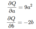
Q. 왜 external_grad가 필요한가?
Autograd에서 미분(differentiation)
autograd 가 어떻게 변화도(gradient)를 수집하는지 살펴보겠습니다. requires_grad=True 를 갖는 2개의 텐서(tensor) a 와 b 를 만듭니다. requires_grad=True 는 autograd 에 모든 연산(operation)들을 추적해야 한다고 알려줍니다.
import torch

a = torch.tensor([2., 3.], requires_grad=True)
b = torch.tensor([6., 4.], requires_grad=True)
이제 a 와 b 로부터 새로운 텐서 Q 를 만듭니다 We create another tensor Q from a and b.
Q = 3*a**3 - b**2
이제 a 와 b 가 모두 신경망(NN)의 매개변수이고, Q 가 오차(error)라고 가정해보겠습니다. 신경망을 학습할 때, 아래와 같이 매개변수들에 대한 오차의 변화도(gradient)를 구해야 합니다. 즉,
Q 에 대해서 .backward() 를 호출할 때, autograd는 이러한 변화도들을 계산하고 이를 각 텐서의 .grad 속성(attribute)에 저장합니다.
Q 는 벡터(vector)이므로 Q.backward() 에 gradient 인자(argument)를 명시적으로 전달해야 합니다. gradient 는 Q 와 같은 모양(shape)의 텐서로, Q 자기 자신에 대한 변화도(gradient)를 나타냅니다. 즉
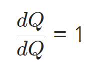
external_grad = torch.tensor([1., 1.])
Q.backward(gradient=external_grad)
이제 변화도는 a.grad 와 b.grad 에 저장됩니다.
# 수집된 변화도가 올바른지 확인합니다.
print(9*a**2 == a.grad)
print(-2*b == b.grad)

'AI TECH' 카테고리의 다른 글
| torch.tensor와 torch.Tensor의 차이 (0) | 2022.09.26 |
|---|---|
| [2주차] Pytorch 프로젝트 (0) | 2022.09.26 |
| CNN의 역전파 (0) | 2022.09.22 |
| [1주차] Python&Math : Generator, Asterisk, 가변인자 (0) | 2022.09.20 |
| [1주차] Python&Math (0) | 2022.09.20 |